

Keep your data assets under control with Aiven's metadata parser
Data's journey in modern companies is usually long, with several steps across different technologies. From source applications storing it in backend databases, passing by batch or streaming technologies for transformation and distribution, data assets arrive at the target systems where they are used in the decision-making process or fed back to the application in reverse ETL (Extract Transform and Load) scenarios.
Keeping track of every step in this fragmented scenario is a tedious process, usually performed manually as part of the documentation effort. But with many fast-moving parts, losing the global view is very easy. When this happens, implications for companies can include duplicated efforts, GDPR violations, and security issues.
The reply to questions like "Who can see this column/table/object" should come from a query in seconds/minutes rather than from a human trying to browse 200+ pages of documentation. Therefore we need to automate the collection of data assets' journeys in a common queryable format as much as possible.
The hidden gold of metadata
How can we automatically extract information about the data? A lot of this information is actually in the metadata!
If we take PostgreSQL® as an example, we can get a long way by scanning the tables in the information_schema. Querying the columns, pg_tables, pg_user, and role_table_grants provides us an overview of which users can see which columns in which tables. Adding a smart parsing of the description field in pg_views also allows us to take one step further and track data transformations happening within the database itself.
Similar discussion can be made for intermediate technologies like Apache Kafka®, where the metadata stored in topic descriptions, ACLs, schema definitions, and connector configurations allows us to create a map of where the data is coming from and where it is going. Or Apache Flink® where we can understand the source and target of each data pipeline.
Different technologies, different languages
If all the data journey stays in a single technology, then the problem is solved! A bit of metadata parsing on the single catalog views/tables, and we have the end-to-end map. But, as discussed above, this is usually not the case. Even more, different technologies will have different objects and attributes defining a data assets: for PostgreSQL, we might talk about tables and columns, while for Apache Kafka, it's topics, schemas and connectors, and in OpenSearch® is namespaces and indexes.
A common abstraction: graph theory
Therefore, if we want to collect, merge, and make available metadata having different shapes, we need to take one step back and abstract our definition of data assets. This is where graph theory becomes handy, allowing us to define each object as a node, and each connection amongst objects as an edge.
- a database? It's a node
- a table? It's a node + an edge to the database it belongs to
- a column? It's a node + an edge to the table it belongs to
- a user? It's a node + an edge to the database it belongs to + an edge to every node it can query/view/edit
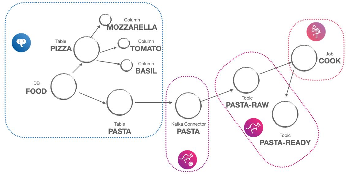
- an Apache Kafka source connector? It's a node + an edge for every source of data + an edge for every destination topic
Storing our assets as nodes/edges allows us to add custom attributes to each entity, using the object properties like the retention time for a topic or the SQL definition for a database view. Even more, it allows us to connect the dots between different technologies! We can, as an example, link the PostgreSQL tables where an Apache Flink® job gets its data from, with the Apache Kafka topic where it lands the transformed assets. If we are diligent and work with Avro and the Karapace schema registry, we might also be able to connect the source to target columns for a complete data lineage.
Sounds difficult, how to do it? Welcome to the metadata parser
Parsing several different technologies and extracting the metadata as node/edges is indeed not a trivial task, requiring you to write a bunch of code to call REST API endpoints, query database tables, or send HTTP requests and merge the output together. However, if you're using Aiven services, we have a nice present for you: the metadata parser, an open-source project built on top of the Aiven's client, which allows you to parse the services belonging to an Aiven project and create a network map of the data assets.
Get the metadata-parser to work
To run the metadata parser on top of your project, you need the following prerequisites:
- Python 3.7+
- a valid Aiven account
- the name of the project that you want to parse
Once collected the above, you can follow these steps:
-
Clone the metadata parser repository and navigate in the
metadata-parserfolder.Loading code... -
Install the required libraries.
Loading code... -
In the
conffolder, copy theconf.env.samplefile toconf.env. Add theTOKENandPROJECTparameters with a valid authentication token and the name of the project to parse. -
If the project doesn't have any running services, you can use the
scripts/create_services.sh <PROJECT_NAME>script to create some temporary services for testing (it requires additional tools likeksql,psqlandmysqlto create data assets correctly).
Run the main.py file to collect metadata from the project.
Loading code...
The above command will parse the project and create:
-
A file
nx.htmlcontaining the complete interactive graph. -
A file
graph_data.dotcontaining the information in DOT format. -
A file
graph_data.gmlcontaining the information in GML format.
If you want to have an interactive view that allows you to filter on a single node and check all dependencies, you can run:
Loading code...
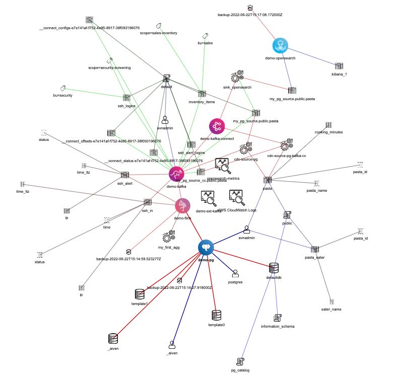
app.py reads the graph_data.gml file generated in the previous step and creates a Reactive Web Application with Plotly and Dash, allowing you to analyze the graph and filter for particular node types or names. The filtering will then show the subgraph connected to the node(s) you're filtering by. You can reach the Dash app at http://127.0.0.1:8050/.
Congrats! You now have the full map of your data assets, spanning different technologies, as a queryable graph!
Just remember, if you want to remove the test services created in step 4, run scripts/delete_services.sh <PROJECT_NAME>.
Wow, can I use it?
Now, think about your questions:
- Data lineage - Where is this column coming from?
- GDPR assessments - Who can see this piece of data? How is my data manipulated?
- Security audits - What user can edit this dataset?
- Impact assessments - What happens if I remove X?
You can now answer these with the graph produced by the metadata parse and some network queries.
We would love people to start using the project, and even more: the metadata parser is a fully open-source project, so we welcome contributions! The project is at the initial stage, therefore we could cover more tools, dig more in-depth into the existing ones, or create alternative ways of parsing and displaying the results.
Some links that you might find helpful:
- Graph theory: to understand how different entities are mapped as nodes, attributes, and edges.
- Aiven Command Line Interface: the Aiven CLI, written in Python, is used to explore services and retrieve metadata; review the methods used to parse the Aiven project.
- Aiven API documentation: to review the list of APIs used by the Aiven Command Line Interface.
- Metadata parser contributing guidelines: to understand how you can contribute to the project.
