


Have you ever wondered how to implement things like an employee record that can show whether an employee is a current employee or has left the company? Using most standard databases, this can become cumbersome: you end up needing to add a new line to your database every time an employee’s status changes.
Bitemporal data can solve that problem, by allowing you to update one record and query the record’s status as it changes through time. This lets you model your database in a way that corresponds to your actual business, rather than a way that suits your database.
To learn more about implementing a bitemporal data model with Postgres, read on for a post from a guest contributor, Henrietta (Hettie) Dombrovskaya!
What is bitemporal data?
If this is the first time you’ve come across the expression bitemporal data, you might be puzzled: time is already considered the fourth dimension, so how can you have more than one time? Before we get more confused, let's take a moment to talk about temporal queries and adding time to data in general.
Bitemporal data lets us query changes against a particular piece of data as it changes through time, all in the same record in the database. This is useful for things like employee records (as mentioned above), options trading, and any environment where auditing is a requirement.
The idea that we should be able to query data at a point in time has been very popular since the dawn of databases. Wouldn't it be nice, for example, in addition to being able to query the current state of things, to query things like:
Loading code...
Wouldn't it be nice to run the same query for any date in the past, like this:
Loading code...
Or, maybe, something like this:
Loading code...
All of these queries reference a specific point in time ("September 1, 2022") or are related to a point in time ("when did John Smith become a manager"). All of these are extremely useful… and none are supported by regular SQL.
Temporal data is the idea that data changes over time. HR records are an example of this, as an employee's status with the company (employed, no longer employed) changes through time.
Another use case for temporal data is auditing. Imagine we have a financial report which gives us the revenue for the past six months. We know what the numbers looked like yesterday. Today, we ran the same report, and the numbers for the past month look different.
What happened? Apparently, somebody changed some numbers in the database. If we were wise, we have audit tables and triggers that record all modifications in historical tables and could investigate this case and find out when the changes were made. If we weren’t, we have a serious issue on our hands.
However, we won't be able to go back in time and rerun the same report as it looked a week ago. Restoring data to a point in time in another environment is a slow process and can't be done on the fly.
We could achieve both of these use cases using a temporal database. A temporal database understands the data in it through time, rather than in a single current state.
For a long time, conversations about temporal databases were purely theoretical: they were considered to be too complicated to implement, and so any such implementation was deemed inefficient or too space-intensive. The pg_bitemporal project is the one that successfully addresses both classes of problems in one comprehensive solution.
How bitemporal data works
Bitemporal data and its implementation in databases are based on the works of Johnson and Weis’ Asserted Versioning Framework (AVF). The Asserted Versioning Framework is a way to operate on data in two-dimensional time.
The most important feature of AVF is bitemporality: each row in a bitemporal table is associated with two temporal intervals: effective time and asserted time.
Effective time defines when the data contained in a row is valid. For example, “John Doe will become our customer on June 1, 2022” has an effective start date of June 1, 2022. We don’t know the end date, so we can assume this statement has an effective end date far in the future. For the purposes of our database, we can set the effective end date to January 1, 2999. Effective time is bound by the real-world business requirements: when John Doe actually becomes or ceases to be our customer.
Asserted time is the time period in which the data in the row is true. For example, “John Doe will become our customer on June 1, 2022 and will stop being our customer on January 1, 2999” is true from May 1, 2022 to January 1, 2999. Unlike effective time, asserted time isn’t based on real-world requirements, but is based on the period of time we care about observing.
Given the above, this is what the bitemporal insert looks like on a graph. The infinity sign means “forever in the future”. The bitemporal insert is the area on a graph defined using the effective time and asserted time as bounding axes:
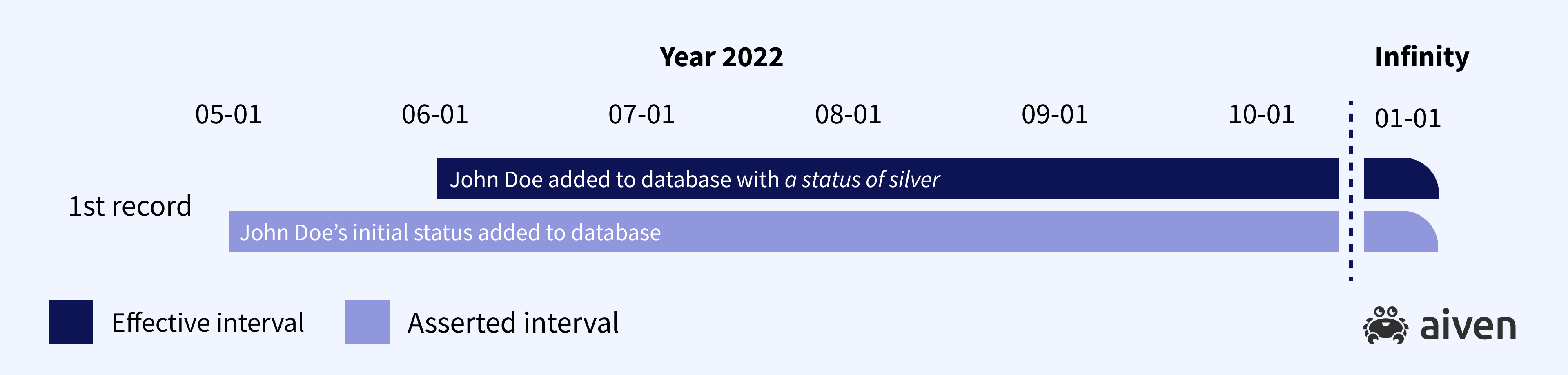
Now let’s imagine that our data model has some additional data, for example a customer status. “John Doe will become our customer on June 1, 2022, with an initial status of Silver.” is true between May 1, 2022 and January 1, 2999.
Now let’s update John Doe’s customer status: “John Doe will become our customer on June 1, 2022, with an initial status of Silver. On September 15, 2022, John Doe’s customer status updated to Gold.”
What happens to our asserted dates in this case? Well, we end up with three statements that are true in different circumstances:
-
“John Doe will become our customer on June 1, 2022, with an initial status of Silver.” is true between May 1, 2022 and January 1, 2999.
-
“John Doe is our customer as of June 1, 2022, with an initial status of Silver” is true between June 1, 2022 and January 1, 2999.
-
“John Doe is our customer as of June 1, 2022, with a status of Gold” is true between September 15, 2022 and January 1, 2999.
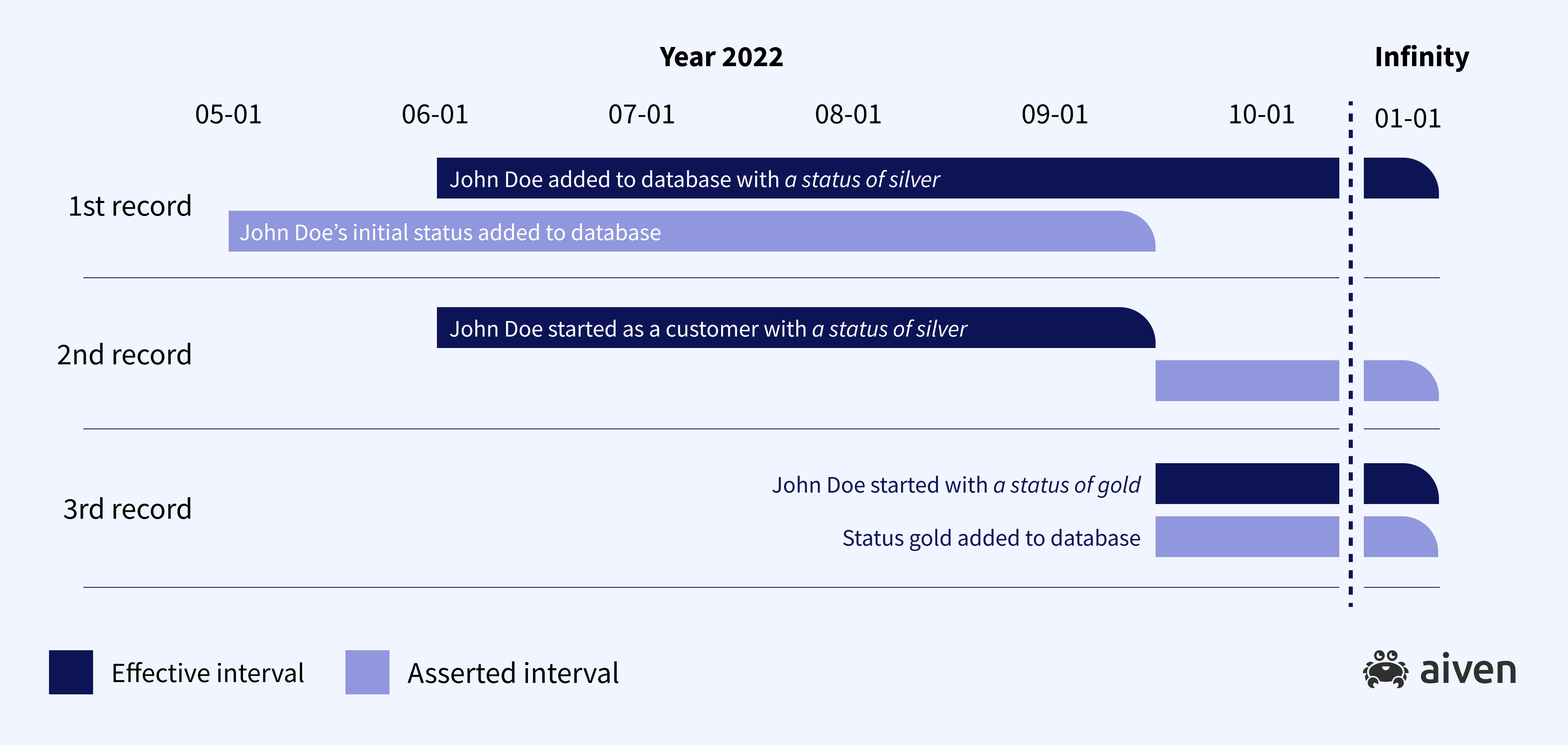
This kind of record update is called a bitemporal update. The previous record (with customer type Silver) is not no longer true for our asserted time. Now we have two historical records, both asserted starting from September 15, 2022 (see Figure 2)
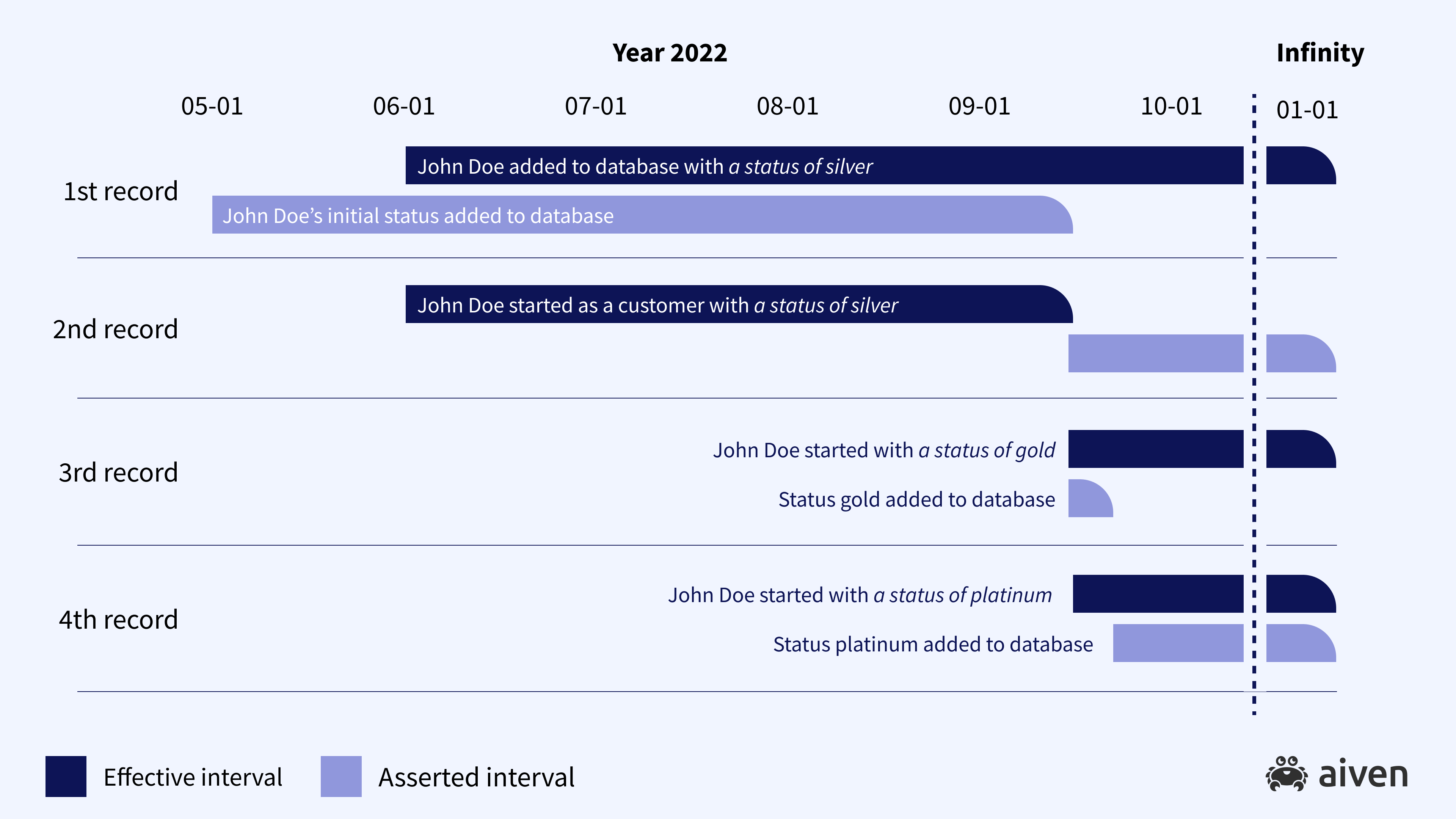
Now, if a week later we realize that we made a mistake and the correct type change should have been for Platinum, not Gold, we can execute a bitemporal correction as presented in Figure 3. Now, we currently assert that John Doe’s customer type is Platinum now and previously was Silver. But if we go back to any date between September 15 and September 22, we will see a different history – first Silver and then Gold.
Now the following is true of our data:
-
“John Doe will become our customer on June 1, 2022, with an initial status of Silver.” is true between May 1, 2022 and January 1, 2999.
-
“John Doe is our customer as of June 1, 2022, with an initial status of Silver” is true between June 1, 2022 and January 1, 2999.
-
“John Doe is our customer as of June 1, 2022, with a status of Gold” is true between September 15, 2022 and January 1, 2999.
= “John Doe is our customer as of June 1, 2022, with a status of Platinum” is true between September 22, 2023 and January 1, 2999.
The pg_temporal project
Now, let me introduce to you the pg_bitemporal project – a PostgreSQL-based implementation of AVF that works!
The GitHub repo contains the SQL files with the source code, and the _load_all.sql script installs it for you. The /doc directory contains references and several PowerPoint presentations and recordings, and the/tutorial directory contains bitemporal tutorial.
Why implement this using PostgreSQL?
Now that we understand more about how bitemporal data works on a conceptual level, we can see why it’s difficult to implement: each row in our bitemporal database needs to essentially have its own table for data over time.
So how do we go about implementing AVF? Well, the pg_temporal project chose PostgreSQL.
PostgreSQL has several features which are critical to make implementation of AVF a success:
-
Range type support allows defining effective and asserted as timestamp with timezone ranges, thus having only two columns instead of four. Moreover, there are multiple operations defined for time-ranges, like includes and overlaps.
-
Infinity (+/-) is a special value that is greater than any other value (works for all numeric and DateTime types); we use it to indicate the "current" time range.
-
GIST indexes and GIST with exclusion constraints.
Learn more with a tutorial
You can learn how to use temporal data with this tutorial. In the tutorial, we build an example bitemporal schema using the following: customer, staff, order and order_line tables. Then, we follow a typical business process: a customer places an order, and then, several changes occur: a customer changes their phone number, a staff is moved to a new location, a product price changes. The tutorial explains when to use bitemporal update, and when - bitemporal correction. It also demonstrates how easy it is to execute different historical queries using the pg_bitemporal.
About the author
Henrietta (Hettie) Dombrovskaya (currently a Database Architect at DRW) is a database researcher and developer with over 35 years of academic and industrial experience. She holds a Ph.D. in Computer Science from the University of Saint Petersburg, Russia. She taught Database and Transaction theory at the University of Saint - Petersburg (Russia), and at the Computer Systems Institute in Skokie, IL as well as multiple database tuning classes for both beginners and advanced professionals.
Henrietta is very active in the PostgreSQL community. Starting from January 2017 she leads the Chicago Postgres User Group and she regularly talks at the PostgreSQL conferences. Her contributions to the community include the pg_bitemporal project, postgres_air training database, and the NORM technology.
To get the latest news about Aiven for PostgreSQL and other services, plus a bit of extra around all things open source, subscribe to our monthly newsletter! Daily news about Aiven is available on our LinkedIn and Twitter feeds.
