Image recognition with Python, OpenCV, OpenAI CLIP and pgvector
Vector embeddings are key to ML, and here we describe how to use OpenCV, OpenAI CLIP and pgvector to generate vectors and use them to perform image recognition on a corpus of photos.
Vector embeddings are key to ML, and here we describe how to use OpenCV, OpenAI CLIP and pgvector to generate vectors and use them to perform image recognition on a corpus of photos.
In the era of AI anything is a vector: from huge texts being parsed and categorized by Large Language Models (LLMs) to images being decomposed to find specific objects in them.
When asking questions to these models, the answer is defined by proximity: the set of stored vectors is parsed to find out the closest one (or set) in terms of distance, angle or similar metric.
If the entire vectorised dataset can be hosted in memory, no problem; but what happens when data gets big? This is where solving the problem with tools that are aimed at storing huge datasets can help, even better if they expose the search functionalities in a known language (SQL) and without the need to extract the entire dataset each time. In our case the tool is PostgreSQL® and the vector functionality is provided by the pgvector extension, newly released in Aiven for PostgreSQL®.
We'll recreate a familiar use-case: you're at an event, and a friend or photograper takes a lot of pictures which are then shared with all the participants. How to identify all the pictures where you are included without having to browse them all? We recently had our yearly face to face meeting at Aiven, called Crab Week, so I had the perfect dataset to start playing with vector representation and search.
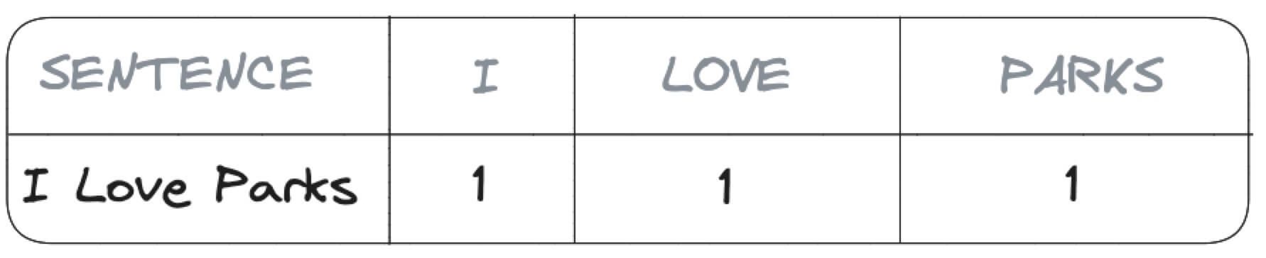
Information can be stored in several ways, just think about the sentence I Love Parks: you could represent it in a table with three columns to flag the presence or not of each word (I, LOVE and PARKS) as per image below:
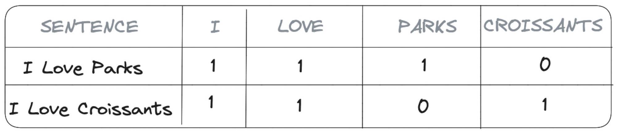
This is a lossless method, no information (apart from the order of words) is lost with this encoding. The drawback though is that the number of columns grows with the number of distinct words within the sentence. For example, if we try to also encode I Love Croissants with the same structure we'll end up with four columns I, LOVE, PARKS and CROISSANTS as shown below.
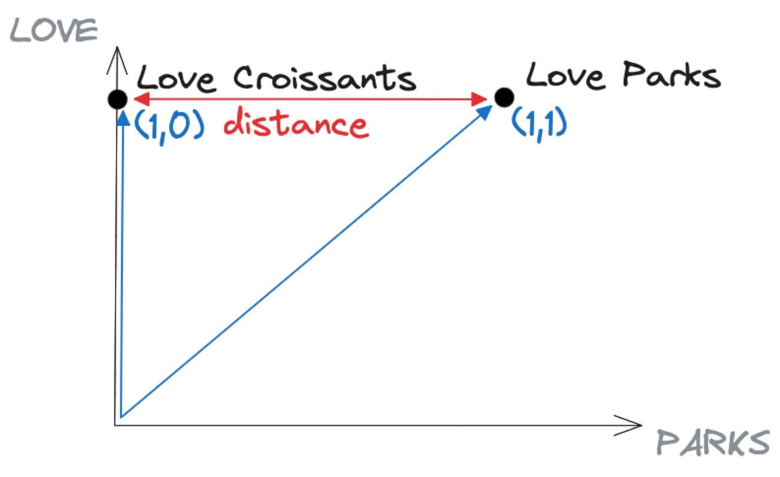
What are embeddings then? As mentioned above, storing the presence of each word in a separate column would create a very wide and unmanageable dataset. Therefore a standard approach is to try to reduce the dimensionality by aggregating or dropping some of the redundant or not very distiguishable information. In our previous example, we could still encode the same information by:
I column since it doesn't add any value (it's always 1)CROISSANTS column since we can still distinguish the two sentences by the presence of the PARK word.If we visualize the two sentences above in a graph only using the LOVE and PARKS axis (therefore excluding the I and CROISSANTS), the result shows that I Love Parks is encoded as (1,1) since it has present both the LOVE and the PARKS words. On the other hand I Love Croissants is encoded with (1,0) since it includes LOVE but not PARKS.
In the graph above, the distance represents a calculation of similarity between two vectors: The more two vectors point to the same direction or are close to each other, the more the information they represent should be similar.
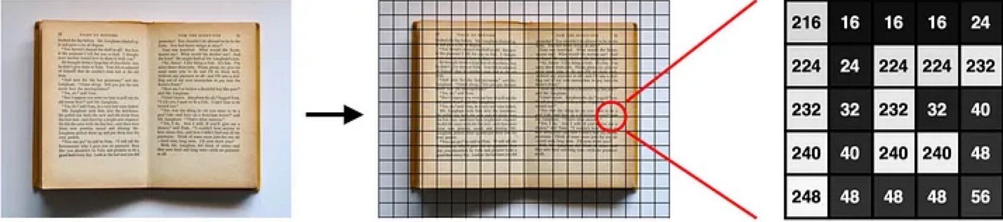
A similar approach also works for pictures. As beautifully explained by Mathias Grønne and visualized in the image below (it's Figure 1.1 from the above blog, original book photo photo by Jess Bailey on Unsplash), an image is just a series of characters in a matrix, and therefore we could reduce the matrix information and create embeddings on it.
pgvectorIf you, like me, use IPhotos on Mac, you’ll be familiar with the “People” tab, where you can select one person and find the photos where this person is included.
I used the following code to do the same sort of thing with the pictures coming from Crab Week - you’re invited to run it, with adaptations, on top of any folder containing images.
Since images are sensitive data, we don't want to rely on any online service or upload them to the internet. The entire pipeline defined below is working 100% locally.
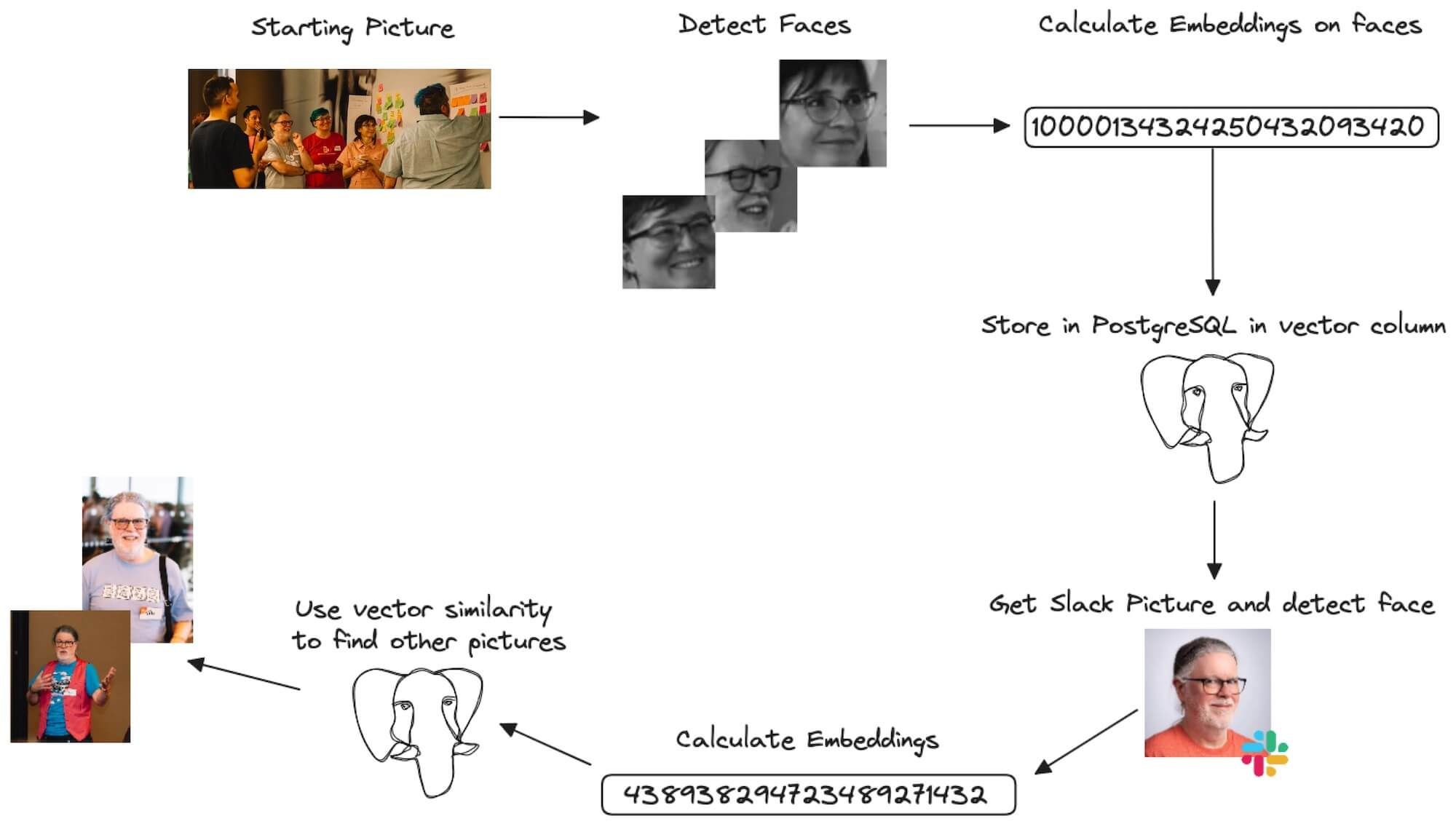
The data pipeline will involve several steps:
vector column from pgvectorpgvector distance function to retrieve the closest faces and therefore photosThe entire flow is shown in the picture below:
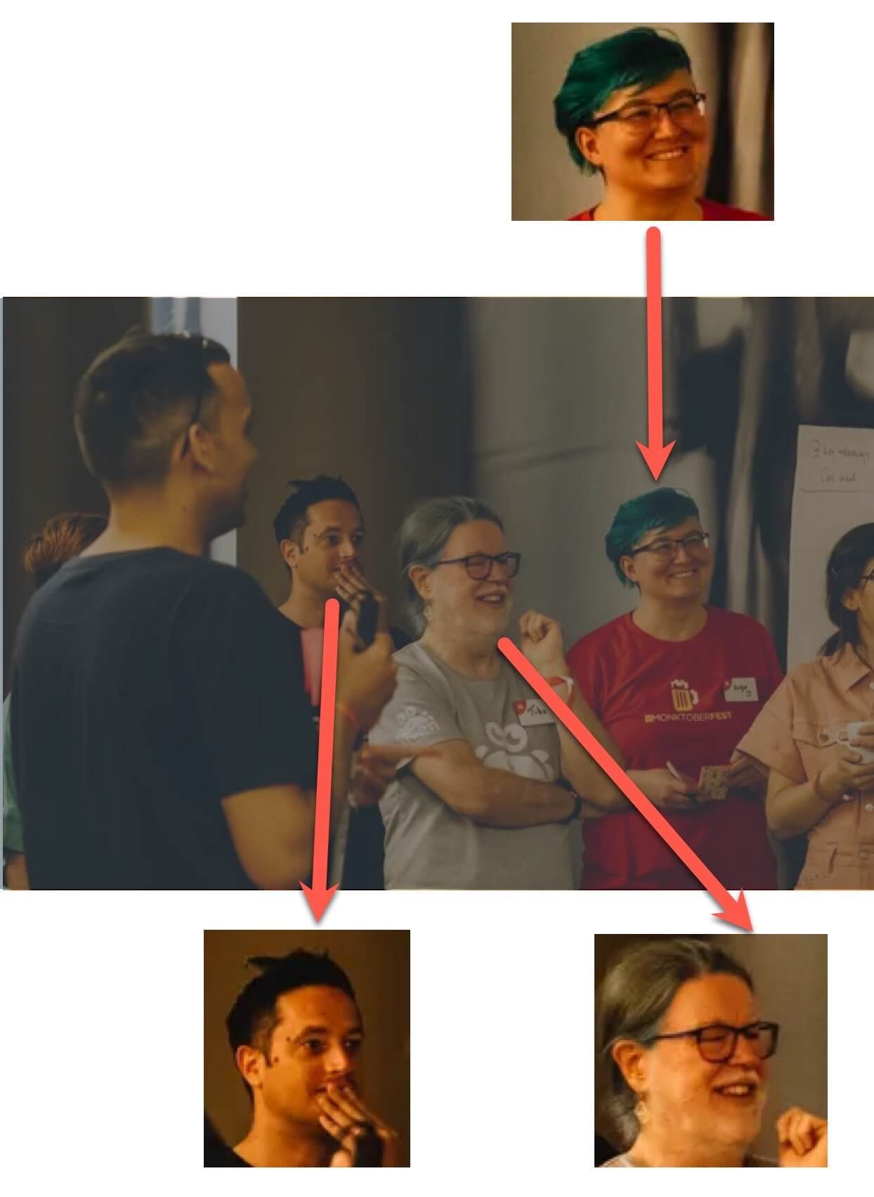
An ideal dataset to calculate embeddings would contain only pictures of one person at a time, looking straight in the camera with minimal background. As we know, this is not the truth for event pictures, where a multitude of people is commonly grouped together with various backgrounds. Therefore, to create a machine learning algorithm that will be able to find a person included in a picture, we need to isolate the faces of the people within the photos and create the embeddings on the faces rather than over the entire photos.
To "extract" faces from the pictures we used Python, OpenCV a computer vision tool and a pre-trained Haar Cascade model, the description of the process can be found in this article.
To get it working, we just need to install the opencv-python package with:
Loading code...
Download the haarcascade_frontalface_default.xml pre-trained Haar Cascade model from the OpenCV GitHub repository and store it locally.
Insert the code below in a python file, replacing the <INSERT YOUR IMAGE NAME HERE> with the path to the image you want to identify faces from and <INSERT YOUR TARGET IMAGE NAME HERE> to the name of the file where you want to store the face.
Loading code...
The line that performs the magic is:
Loading code...
Where:
gray_img is the source image in which we need to find facesscaleFactor is the scaling factor, the higher ratio the more compression and more loss in image qualityminNeighbors the amount of neighbour faces to collect. The higher the more the same face could appear multiple times.minSize the minimum size of a detected face, in this case a square of 100 pixels.The for loop iterates over all the faces detected and stores them in separate files; you might want to define a variable (maybe using the x and y parameters) to store the various faces in different files. Moreover, if you plan to calculate embeddings over a series of pictures, you'll want to encapsulate the above code in a loop parsing all the files in a specific folder.
The result of the face detection stage is not perfect: it identifies three faces out of the four that are visible, but is good enough for our purpose. You can fine tune the algorithm parameters to find the better fit for your use cases.
Once we identified the faces, we can now calculate the embeddings. For this step we are going to use imgbeddings, a Python package to generate embedding vectors from images, using OpenAI's CLIP model via Hugging Face transformers.
To calculate the embeddings of a picture, we need to first install the required packages via
Loading code...
And then include the following in a Python file
Loading code...
The code above calculates the embeddings. The result is a 768 element numpy vector for each input image, representing its embedding.
pgvectorIt's time to start using the capability of PostgreSQL and the pgvector extension. First of all we need a PostgreSQL up and running, we can navigate to the Aiven Console, create a new PostgreSQL selecting the favourite cloud provider, region and plan and enabling extra disk storage if needed. The pgvector extension is available in all plans. Once all the settings are ok, you can click on Create Service.
Once the service is up and running (it can take a couple of minutes), navigate to the service Overview and copy the Service URI parameter. We'll use it to connect to PostgreSQL via psql with:
Loading code...
Once connected, we can enable the pgvector extension with:
Loading code...
And now we can create a table containing the picture name, and the embeddings with:
Loading code...
Check out the embedding vector(768), we are defining a vector of 768 dimensions, exactly the same dimension as the output of the ibed.to_embeddings(img) function in the previous step.
To load the embedding in postgreSQL we can use psycopg2 by installing it with
Loading code...
and then using the following Python code always replacing the <SERVICE_URI> with the service URI
Loading code...
Where file_name and embedding are the variables from the previous Python statement.
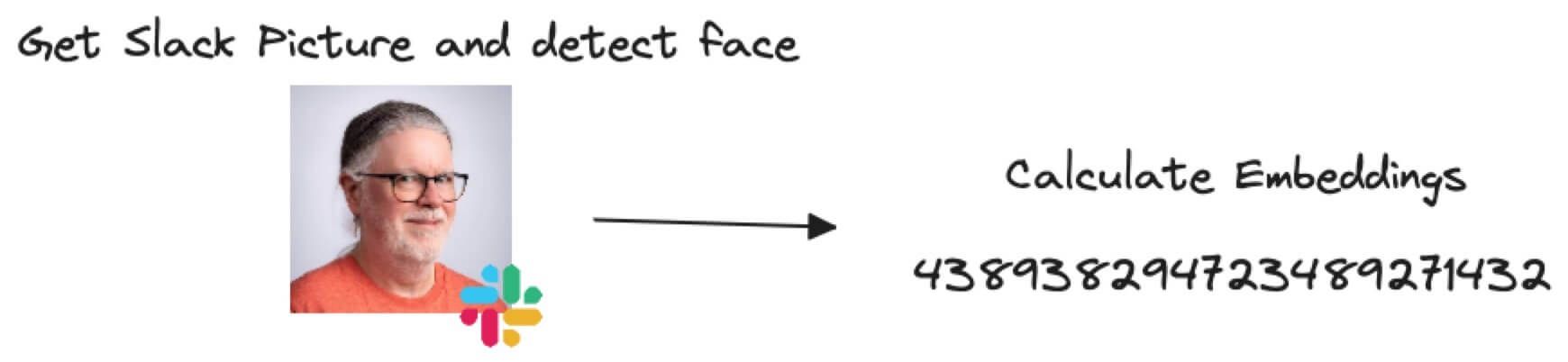
The following steps in the process are similar to the ones already done above, this time the source image is the Slack profile picture where we'll detect the face and calculate the embeddings. The code above can be reused by changing the location of the source image.
The code below can give you a starting point
Loading code...
Since Slack pictures could be complex, the above code has a for loop iterating over all the detected faces. You might want to add additional checks to find the most relevant face to calculate the embeddings from.
The final piece of the puzzle is to use the similarity functions available in pgvector to find pictures where the person is included. pgvector provides different similarity functions, depending on the type of search we are trying to perform.
We'll use the distance function, that calculates the euclidean distance between two vectors for our search. To find the other pictures with closest distance we can use the following query in Python:
Loading code...
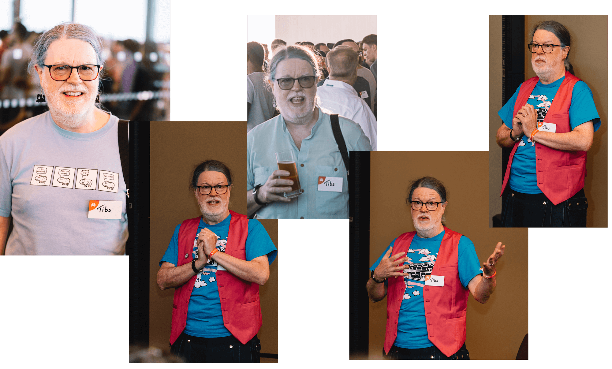
Where slack_img_embedding is the embeddings vector calculated on top of the Slack profile picture at the previous step. If everything is working correctly, you'll be able to see the name of top 5 pictures that are similar to the Slack profile image as input.
The results, in the crabweek case was five photos where my colleague Tibs was included!
Machine Learning is becoming pervasive in our day to day activities. Being able to store, query and analyse data embeddings in the same technology where the data resides, like a PostgreSQL database, can provide a number of benefits in machine learning democratisation and enable new use cases achievable by a standard SQL query.
To know more about pgvector and Machine Learning in PostgreSQL:
Table of contents
pip install opencv-python# import the OpenCV library - it's called cv2
import cv2
# load the Haar Cascade algorithm from the XML file into OpenCV
alg = "haarcascade_frontalface_default.xml"
haar_cascade = cv2.CascadeClassifier(alg)
# read the image as grayscale
file_name = '<INSERT YOUR IMAGE NAME HERE>'
img = cv2.imread(file_name, cv2.IMREAD_GRAYSCALE)
# find the faces in that image
# this gives back an array of face locations and sizes
faces = haar_cascade.detectMultiScale(
    gray_img,
    scaleFactor=1.05,
    minNeighbors=2,
    minSize=(100, 100)
)
# for each face detected
for x, y, w, h in faces:
# crop the image to select only the face
cropped_image = img[y : y + h, x : x + w]
# write the cropped image to a file
target_file_name = '<INSERT YOUR TARGET IMAGE NAME HERE>'
cv2.imwrite(
target_file_name,
cropped_image,
)faces = haar_cascade.detectMultiScale(
gray_img,
scaleFactor=1.05,
minNeighbors=2,
minSize=(100, 100)
)pip install imgbeddings
pip install pillow # import the required libraries
import numpy as np
from imgbeddings import imgbeddings
from PIL import Image
# load the face image from its file
file_name = "INSERT YOUR FACE FILE NAME"
img = Image.open(file_name)
# loading `imgbeddings` so we can calculate embeddings
ibed = imgbeddings()
# calculating the embedding for our image
embedding = ibed.to_embeddings(img)[0]psql <SERVICE_URI>CREATE EXTENSION vector;CREATE TABLE pictures (picture text PRIMARY KEY, embedding vector(768));pip install psycopg2# import the required libraries
import psycopg2
# connect to our database and upload the record
conn = psycopg2.connect('<SERVICE_URI>')
cur = conn.cursor()
cur.execute('INSERT INTO pictures values (%s,%s)', (file_name, embedding.tolist()))
conn.commit()
conn.close()# load the image you want to search with
file_name = '<INSERT YOUR SLACK IMAGE NAME HERE>'
img = cv2.imread(file_name, cv2.IMREAD_GRAYSCALE)
# find the faces
faces = haar_cascade.detectMultiScale(
gray_img,
scaleFactor=1.05,
minNeighbors=2,
minSize=(100, 100)
)
# load `imgbeddings` so we can calculate embeddings
ibed = imgbeddings()
# for each face detected in the Slack picture
for x, y, w, h in faces:
# crop the image to select only the face
cropped_image = img[y : y + h, x : x + w]
# calculating its embedding
slack_img_embedding = ibed.to_embeddings(cropped_image)[0]conn = psycopg2.connect('<SERVICE_URI>')
cur = conn.cursor()
string_representation = "".join(str(x) for x in slack_img_embedding.tolist())
cur.execute("SELECT picture FROM pictures ORDER BY embedding <-> %s LIMIT 5;", (string_rep,))
rows = cur.fetchall()
for row in rows:
print(row)