



TL;DR
- Inference, running a finished model, is where almost all the engineering work in an LLM system lives, and most of it is data engineering you already know.
- A retrieval pipeline uses two models: a small encoder that turns text into vectors to find the right documentation, and a decoder that writes the answer.
- The specialisation lives in the system, not the model: retrieval (RAG) beats fine-tuning on documentation because it stays current and can cite its sources.
- Quantisation shrinks a 7B model from 14 GB to about 4 GB and makes generation faster, at a small cost in multi-step reasoning.
Part 0 of a three-part series on building a documentation assistant with Aiven. This part gives you the vocabulary. Part 1 is the architecture. Part 2 builds the thing.
Almost everything written about large language models explains how models get built. Very little explains what happens the other billion times, when a finished model sits there answering questions. That second thing is called inference, and it is where practically all of the engineering work actually lives.
Here is the good news for builders who run databases, streams and APIs for a living: inference is much closer to your existing job than the vocabulary suggests. The model is a box that turns bytes into bytes. Everything around it, getting the right data in front of it, keeping latency tolerable, knowing what it did and whether the answer was any good, is work you have done before under different names.
So let's do the vocabulary properly, by following one real question about Apache Kafka® all the way through:
"How do I add partitions to a Kafka topic?"
Every term shows up at the moment it starts to matter. By the end you will know what the words mean and, more usefully, where each one sits in a system that works.
Four words people use interchangeably
Start here, because these four get swapped around constantly and they describe completely different activities.
Training: building a model from nothing. Start with random numbers, show it enormous amounts of text, adjust the numbers until it predicts text well. Those numbers are the weights.
Training a frontier-scale model costs millions of dollars and weeks of GPU time, and only a handful of organisations do it.
Fine-tuning: taking a trained model and adjusting its weights further on a smaller, targeted dataset.
Cheaper than training by orders of magnitude, but still a training job. You need labelled data, GPUs, and you end up with a new set of weights.
Inference: running a finished model. Bytes in, bytes out, weights untouched.
One training run is followed by billions of inferences. That ratio is why inference dominates both the cost and the engineering effort of anything actually deployed.
Serving: the infrastructure that makes inference available. The endpoint, the queue, the batching, the timeouts, the retries.
This series builds the last two and does no training at all. That is a deliberate choice rather than a limitation, and it is worth understanding why, so we come back to it later.
There isn't one model, there are two
This is the distinction most explanations skip, and skipping it is why these systems end up feeling like magic.
- Encoder: reads text, returns a list of numbers. Nothing readable, just coordinates.
- Decoder: reads text, writes text. This is what people mean when they say "LLM".
Our pipeline uses both, and they have almost nothing in common. Encoders are small, fast, and perfectly happy on a CPU. Decoders are large, slow, and produce their output one piece at a time.
They also do different jobs. The encoder finds the right documentation. The decoder writes the answer. Different costs, different latency, different ways of going wrong.
And they never talk to each other directly. The encoder's numbers are only ever used to find passages. What reaches the decoder is the plain text of those passages. The two models are connected by text, nothing else, and that is exactly what lets you replace either one without touching the other.
Now count the calls, because this is the part that surprises people. The encoder runs once for every fragment of documentation in the entire corpus, so tens of thousands of calls before a single user has asked anything. The decoder runs once per question. The small model does nearly all of the work.
Tokens: the unit of everything
Models don't read characters, and they don't read words either.
- Token: a fragment of a word. In a typical vocabulary, "partition" is one token and "partitions" is two. Rough English conversion: one token is about 0.75 words.
- Vocabulary: the fixed list of tokens a model knows, usually tens of thousands of entries. Common words get a token of their own. Rarer ones get split into pieces the model does know.
Every token in the vocabulary has a number, its position in that list. And every model ships with its own vocabulary, so the same sentence splits differently, and gets entirely different numbers, depending on which model reads it. Hold on to both details, because the next section starts from them.
Tokens matter for three separate reasons. They are the billing unit of every hosted model. They are the unit of the size limit. And they set your speed, because a decoder emits output one token at a time.
Context window: the maximum tokens a model can hold at once. Everything counts towards it: your instructions, the documentation you supplied, the conversation so far, and the answer being written.
Go over the limit and nothing degrades gracefully. You get a failure or a truncation.
- Prompt: the text going in.
- Completion: the text coming out.
Those two behave completely differently, and understanding the difference will change how you design.
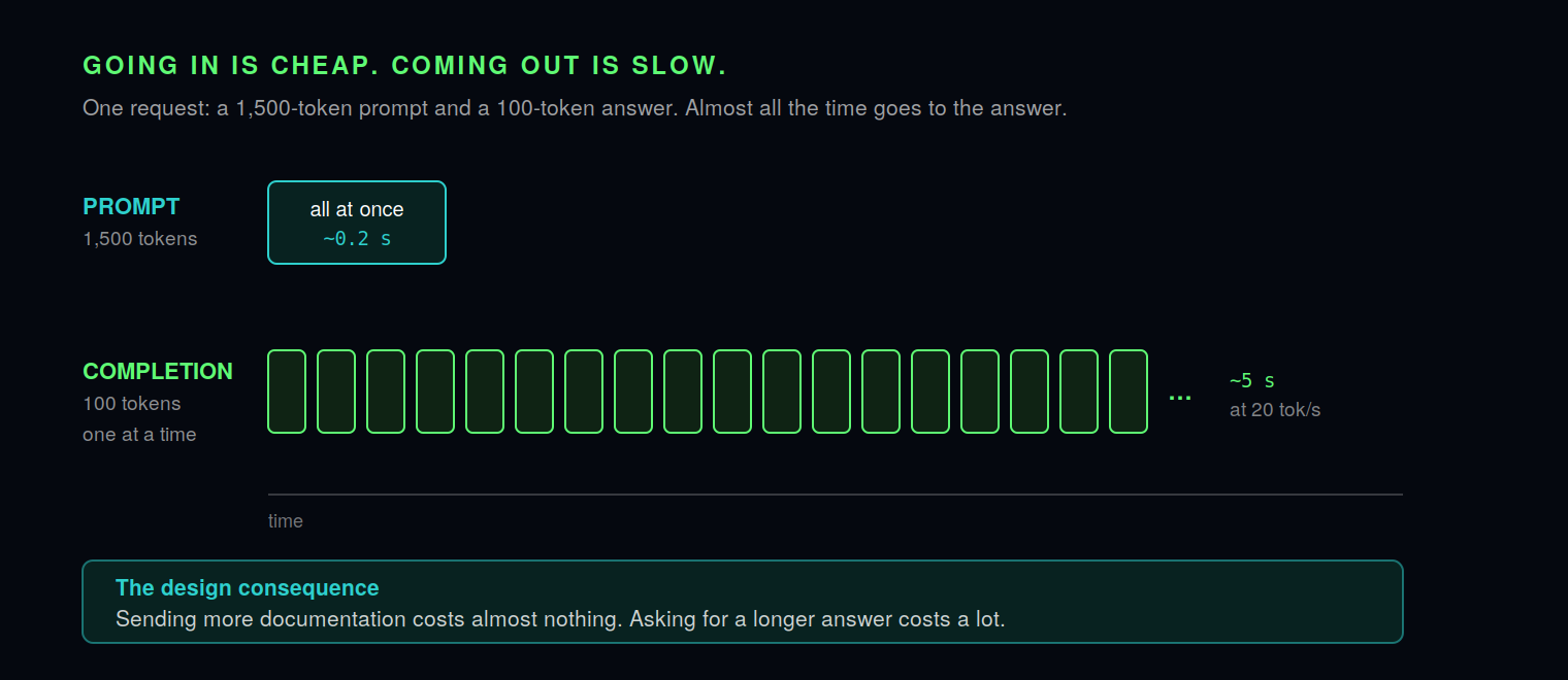
Prompt tokens get processed in parallel, so they are fast. Completion tokens are generated in sequence, so they are slow. A request with a 1,500-token prompt and a 100-token answer spends nearly all its time on those hundred tokens.
Which gives you a rule you can act on immediately: sending more documentation is close to free. Asking for a longer answer is expensive.
Embeddings: teaching a search engine what you meant
Type "how do I add partitions to a topic" into a keyword search and it looks for those exact words. Meanwhile a page titled "increasing partition count on an existing topic" answers the question perfectly and shares almost no words with it. Keyword search walks straight past.
So here is the trick. Feed text to an encoder and you get back a few hundred numbers.
Embedding (or vector): the list of numbers an encoder returns for a piece of text. On its own it means nothing to you. What matters is that texts with similar meaning come back with similar lists.
Which raises the obvious question: how does a list of numbers end up capturing meaning? It is worth a few minutes, because once you have seen it, the rest of the pipeline stops feeling like magic.
How the numbers get made
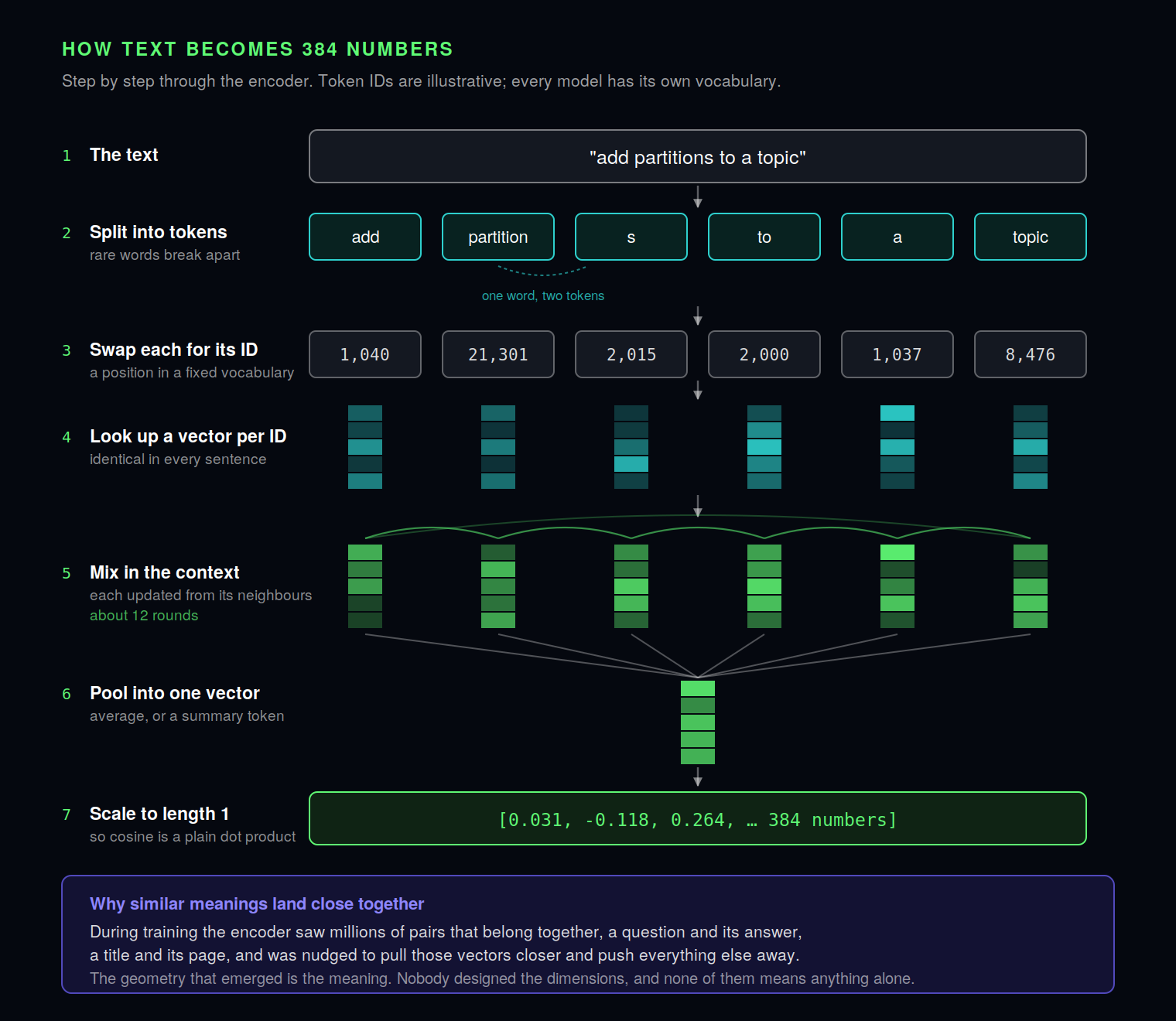
The text gets split into tokens, exactly as in the previous section. "Partitions" comes apart into two.
Each token becomes an ID, its position in the model's vocabulary. Nothing clever yet. It is a dictionary lookup.
Each ID becomes a vector. The model holds a large table with one row of numbers per vocabulary entry, learned during training. At this stage "partition" gets exactly the same vector whether you are talking about a disk or a Kafka topic.
Then the context gets mixed in, and this is the step that matters. The model runs about a dozen rounds in which every token's vector is updated using the vectors of the tokens around it. After those rounds, "partition" sitting next to "topic" and "Kafka" has drifted somewhere quite different from "partition" sitting next to "disk" and "format". Same word, different meaning, different coordinates.
The token vectors get combined into one. Some models average them. Others, bge-small included, put a special summary token at the start of the text and keep its final vector.
Pooling: collapsing one vector per token into a single vector for the whole text.
Finally the vector is scaled to length 1, so that comparing two embeddings becomes a single multiplication. That is what you store.
Why similar meanings end up close
The mechanics explain how you get numbers. They don't explain why the numbers mean anything. That part comes from how the encoder was trained.
Contrastive training: showing a model pairs of texts that belong together, a question and its answer, a title and its page, and adjusting it so their vectors move closer while unrelated texts move apart.
Repeat that over millions of pairs and a geometry emerges in which texts about the same thing cluster together. Nobody designed it. There is no dimension meaning "Kafka" and no dimension meaning "configuration". The meaning isn't in any single number. It is in where the whole vector points relative to everything else.
It also means an encoder is only as good as the pairs it learned from. One trained on general web text knows that "partition" and "shard" are related. Whether it knows that user_config and postgresql.conf answer the same question in two different contexts is a different matter entirely, and we come back to it.
What "similar" means, precisely
Picture each embedding as an arrow pointing somewhere in a space with a few hundred dimensions. Two texts about the same thing point in nearly the same direction.
Cosine similarity: the cosine of the angle between two vectors. 1.0 means identical direction, 0.0 means unrelated.
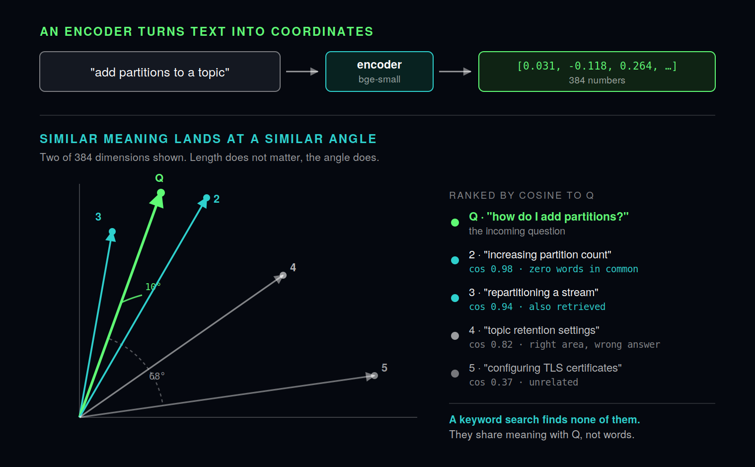
Look at what the diagram is telling you. The question and the two genuinely relevant pages sit within about ten degrees of each other, despite sharing barely a word. The TLS page is sixty-eight degrees away. Finding relevant documentation just became finding the smallest angles, which is a problem databases already solve.
Nearest-neighbour search: finding the stored vectors closest to a query vector. This is why PostgreSQL® with pgvector shows up in every architecture that looks like this one.
The dimension count comes from the model, not from you. A small encoder like bge-small-en-v1.5 gives you 384, which is exactly why the schema in Part 1 has a vector(384) column in it.
And one rule, which is the single most common way these systems fail without telling you: the same model has to embed your documents and your questions. Swap encoders halfway through and you are comparing coordinates from two unrelated spaces. Nothing throws an error. The results quietly stop meaning anything.
What about other languages?
This series sticks to English, deliberately. But the question comes up every time, so here is the short version.
Nothing in the mechanics changes. Tokens, IDs, vectors, context, pooling: all identical. What changes is the training.
Multilingual encoder: an encoder trained on many languages, translation pairs included, so that the same meaning lands in the same place whatever language it is written in.
That is genuinely useful. A question asked in French can retrieve documentation written in English, because "comment ajouter des partitions" and "how do I add partitions" point in nearly the same direction. Quality usually sits a little below same-language search, but it works.
The catch is the vocabulary. Languages that were rarer in the training data get split into more, smaller tokens to say the same thing. More cost per question, less text in the same context window.
And one trap you will recognise by now. The -en in bge-small-en-v1.5 means English. Hand it French and it won't complain. It will chop the text into fragments and return a vector, and that vector will be poor. No error, just quietly worse results.
It is tempting to fix that with a language detector up front, routing each question to an encoder specialised in its language. Resist it. Every encoder has its own space, so a French-specialised vector cannot be compared with English-embedded documents at all. And language detection is at its least reliable on short technical questions full of English jargon, so every misdetection would silently break retrieval. One multilingual encoder for documents and questions alike is simpler, and it fails far more gently.
The general rule is worth keeping beyond this example: put probabilistic decisions where their mistakes are cheap.
One question, start to finish
Time to put the whole thing together.
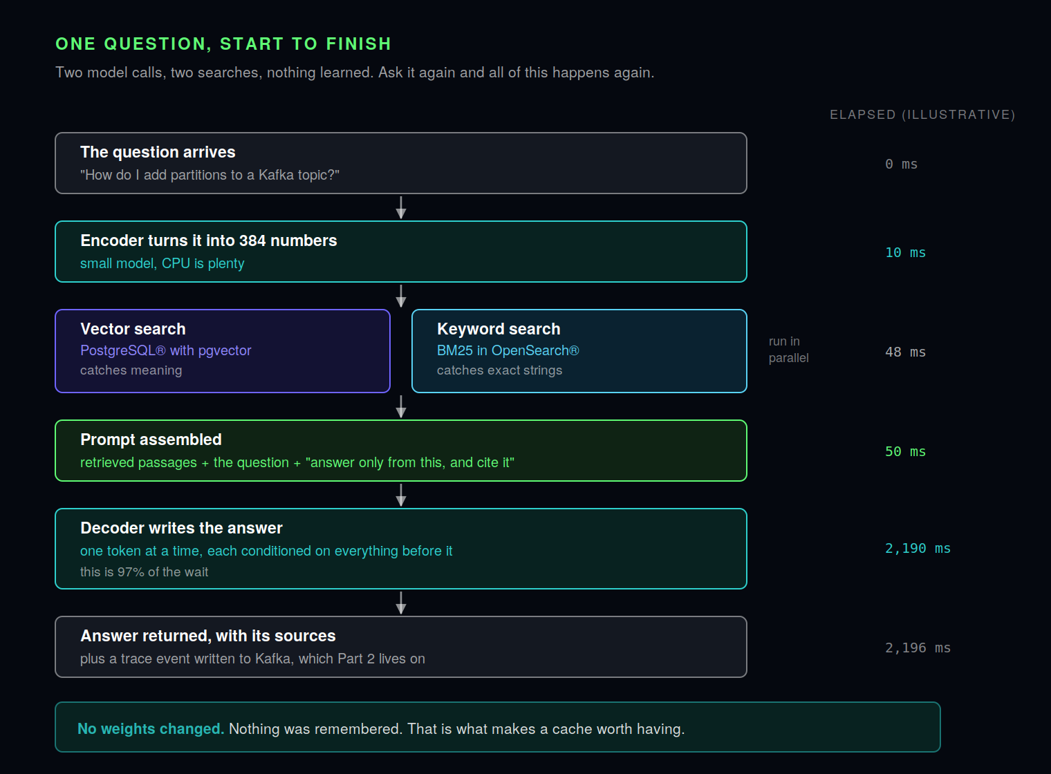
Illustrative timings for a CPU encoder and a local GPU decoder. Part 2 publishes measured figures.
Walking through it:
The question arrives. How do I add partitions to a Kafka topic?
It gets embedded. The encoder turns it into 384 numbers. Around ten milliseconds on a CPU in a typical setup.
Two searches run at once. The vector search finds the fragments pointing in nearly the same direction. Alongside it, a keyword search in OpenSearch® does literal matching, because vector search is good at meaning and bad at exact strings. A question mentioning kafka-topics.sh or a specific error code needs both.
Hybrid retrieval: running vector and keyword search together and merging the results. It reliably beats either one alone.
The prompt gets assembled. The retrieved fragments, the question, and instructions along the lines of: answer only from the documentation below, cite which fragment you used, and say so if the answer isn't in there. About 1,500 tokens now.
The decoder generates. One token at a time, each one conditioned on everything before it. It stops at a length limit or at a stop sequence. In this example it accounts for about 97% of the wait.
The answer comes back, carrying the identifiers of the fragments behind it.
That whole path is one inference request. Two model calls, two searches. No weights changed. Nothing was learned or remembered. Ask the identical question a second time and identical work happens all over again, which tells you immediately that a cache is going to pay for itself.
That has a name: RAG
What you just followed is the pattern everyone calls RAG.
RAG (retrieval-augmented generation): fetching relevant passages from your own data at question time and placing them in the prompt, so the model answers from them rather than from memory.
A small historical note, because it trips people up. The term comes from a 2020 research paper, and in that paper the retriever and the generator were trained together, as one system. That is not what the word means today. Now it almost always means two frozen, off-the-shelf models with a search step between them, which is exactly what this series builds.
The pattern itself is simple enough to fit in one sentence: search, stuff the results into the prompt, generate. That is also why so many tutorials stop there. The trouble is that the hard parts aren't in the acronym.
| The textbook version | What this series builds | |
|---|---|---|
| Search | Vector search only | Vector plus keyword search, because exact identifiers matter |
| Sources | One clean corpus | Aiven docs and upstream docs, which sometimes disagree, with rules for which one wins |
| Indexing | A script you run once | A stream you can replay whenever documents or the encoder change |
| Answers | Whatever the model writes | A citation behind every claim, and a refusal when nothing relevant was found |
| Repeat questions | Full cost every time | Served from cache |
| Knowing it works | A demo that looks good | Every request traced, answers scored against a test set |
The first column demos beautifully and then gets hard to trust. Documents change underneath it, answers can't be checked, and nobody can say whether last week's tweak made things better or worse.
Each row of the second column is a piece of Part 1. The second row in particular, two correct sources giving different answers, is the problem that makes this system worth writing about.
Three knobs that actually matter
A decoder doesn't pick the next token. It produces a probability for every token in its vocabulary, and something else does the picking.
Sampling: the process of choosing the next token from the probabilities the model produced.
There are a lot of sampling parameters. Three of them matter.
Temperature: scales the probabilities before choosing. At 0, the model always takes the most likely token, so it is deterministic and repetitive. At 1.0, it samples from the raw distribution, so you get variety and mistakes.
For technical support you want 0 to 0.3. The same question should get the same answer, and creativity is a defect.
- Top-p (nucleus sampling): restricts the choice to the smallest set of tokens whose probabilities add up to p. At 0.9, the long tail of unlikely tokens is simply off the table.
- Stop sequence: a string that ends generation. Useful for structured output, and for cutting off a model that has started inventing your next question for you.
Set temperature low, top-p around 0.9, and leave everything else at its default. The rest is mostly noise.
Quantisation: same model, less memory
Quantisation only makes sense once you have a clear picture of what is being quantised. So, one step back first.
What a weight actually is
A weight (or parameter) is a single number the model learned during training. Mechanically, a model is an enormous chain of multiplications and additions, and the weights are the numbers your input gets multiplied by.
You have already met some. That table in the embedding section, one row of numbers per vocabulary entry: every number in it is a weight. So is every number used in the dozen rounds of context mixing. When a model is described as "7B", it means seven billion of these numbers.
Two things follow, and both are worth sitting with.
Training is nothing more than adjusting these numbers, and inference is nothing more than reading them. That is the distinction from the very first section of this article, stated mechanically.
And the model is its weights. The code that runs them is small and generic, broadly the same for thousands of different models. Download a model and what you are really downloading is one very large file of numbers.
Think of them as billions of dials, set once at the factory and never touched again.
Why 16 bits
Every one of those numbers has to be stored, and the question is how precisely.
Precision: how many bits are used to store each number. More bits means more distinct values it can take, and more memory.
Models were originally trained in 32-bit floating point, the standard format for scientific computing, with around seven significant digits. That turned out to be more precision than models need. At 16 bits, roughly three significant digits, they behave essentially the same, while using half the memory and running faster on hardware built for it. So 16 bits became the default. You will see both fp16 and bf16 around: both are 16 bits, they just divide those bits differently between range and detail.
Which gives you the one piece of arithmetic everything else rests on:
Memory for weights = number of weights × bytes per weight.
At 16 bits, two bytes each, seven billion weights come to 14 GB. And that is before the model has done any work at all.
Going lower
Storing weights with fewer bits than they were trained with, typically 8 or 4, is called quantisation.
Here is the part that sounds like it can't possibly work. An 8-bit integer can take 256 distinct values. A 4-bit integer can take sixteen. Sixteen possible values, for every weight in the model.
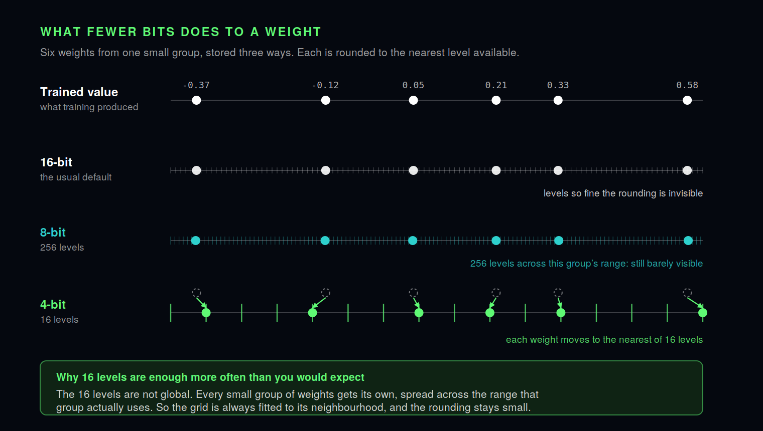
The trick is that those sixteen values aren't the same everywhere. Weights are handled in small groups, and every group gets its own scale: its sixteen levels are spread across the range that group's weights actually occupy. Each weight then rounds to the nearest level. So a weight isn't replaced by one of sixteen global numbers. It is replaced by one of sixteen numbers chosen for its neighbourhood, and the rounding stays small.
It works because no single weight matters very much. Behaviour emerges from billions of them combined, and small rounding errors mostly cancel out. Where it breaks is wherever errors compound: long chains of reasoning, where one slightly-off step feeds the next.
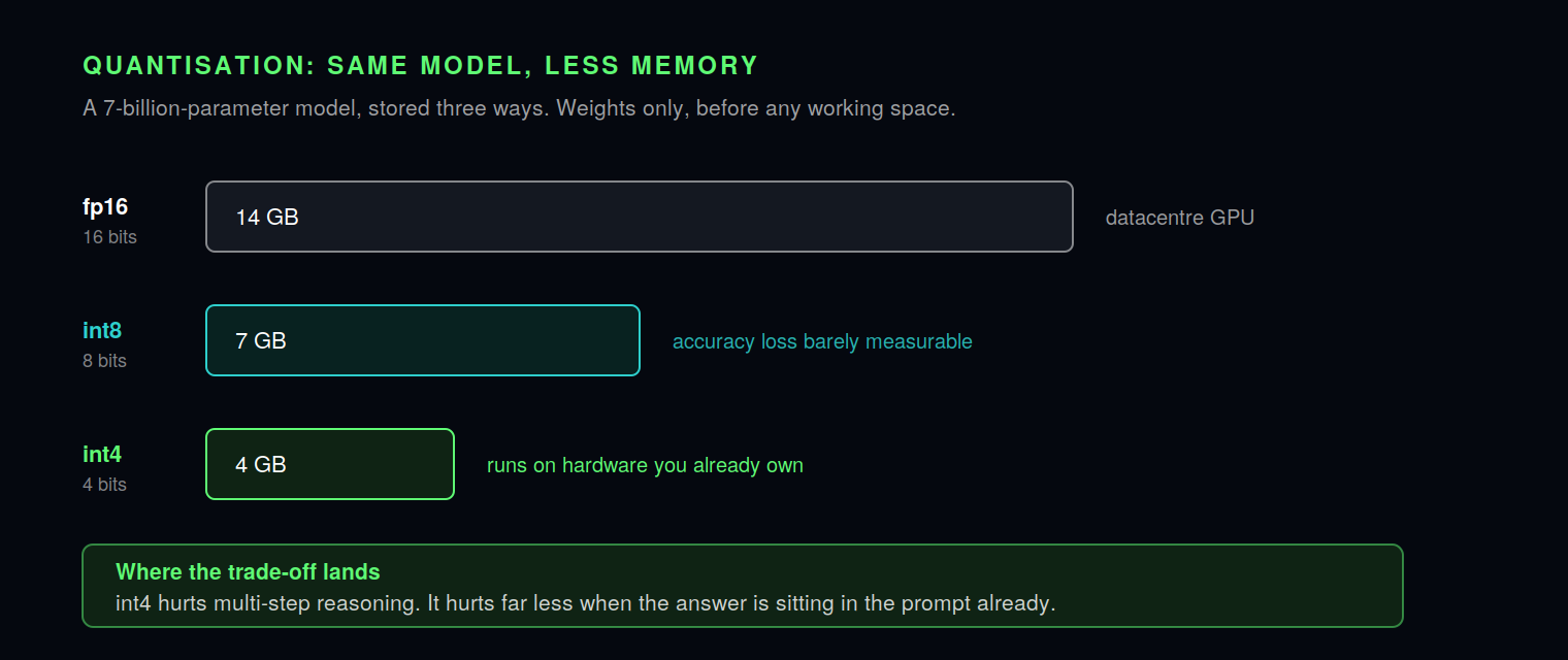
That 4 GB is the whole point. It is 3.5 GB of raw weights plus the per-group scales quantisation has to store alongside them, and it is the difference between needing a datacentre GPU and running on hardware sitting under your desk.
The surprise: smaller is also faster
You would expect a compressed model to be slower, since the weights have to be unpacked before use. For generation, the opposite happens.
To produce each token, the model reads every one of its weights from memory. So generation speed is limited by how fast memory can be read, not by how fast the chip can calculate.
Memory bandwidth: how many bytes per second the hardware can move from memory to the chip. For generating text, this is usually the real bottleneck.
Fewer bytes per weight means fewer bytes to read per token. A rough ceiling: tokens per second ≈ memory bandwidth ÷ model size. On a machine moving 100 GB/s, that is about 7 tokens/s for the 14 GB version and about 25 for the 4 GB one. Real numbers land a little below, because of the unpacking, but the gap holds.
Time to first token barely moves, though. Reading the prompt happens in parallel and is limited by calculation, not by memory. And nothing else changes: same tokenizer, same vocabulary, same context window. The memory you save even leaves more room for the context itself, so longer documents or more simultaneous users fit.
Fewer bits, or fewer weights?
Quantising isn't the only way to shrink a model. You could simply use a smaller one. And both routes can land at the same memory:
| Weights | Bits per weight | Memory | |
|---|---|---|---|
| Large model, quantised | 7 billion | 4 | about 4 GB |
| Small model, full precision | 2 billion | 16 | about 4 GB |
Same budget, two very different models. The first kept its seven billion dials and lost fine detail on each one. The second kept full detail on far fewer dials.
The general finding is that the large model squeezed down usually wins, down to about 4 bits. Below that, quality falls away quickly. That is why int4 is where most local deployments settle, and why a quantised 7B is a far more common sight than a full-precision 2B. And when a task needs better reasoning, reach for a bigger model before reaching for more bits. Going from 4 to 8 bits recovers most of what quantisation costs; going to 16 adds almost nothing at inference time.
For our pipeline the trade is even easier than usual. Int4 hurts most on multi-step reasoning, and least when the model is summarising documentation sitting right there in its prompt. That is exactly our situation, and part of why retrieval pipelines tolerate small models better than general-purpose assistants do.
One misconception worth heading off. Quantisation teaches the model nothing. It is packaging, applied once training is finished. Think of saving a photo as a smaller JPEG: the file shrinks and the image gets slightly less sharp, but what is in the picture doesn't change. Making a model better at medicine, law or Kafka means changing what is in the picture, and that is training or fine-tuning. The two often happen in sequence, specialise first and then quantise to run on your own hardware, but they are separate steps. One changes what the model knows. The other only changes how much room it takes.
One clarification to finish: all of this is about decoders. Encoders are small enough that it rarely comes up. bge-small has around 33 million weights, which at 16 bits is under 70 MB.
Why it feels slow, and what to measure
Two numbers get conflated constantly, and they measure different things.
- Time to first token: how long before the first character appears. Dominated by prompt processing and by whatever ran before the model got called, which for us is retrieval.
- Tokens per second: generation speed after that. A 100-token answer at 20 tokens/s takes five seconds no matter how quickly the first token arrived.
- Throughput: total tokens per second across all concurrent requests. A different axis entirely. Batching improves it and slightly worsens individual latency, because requests wait around to be grouped.
Then there is the one that changes user experience without changing anything technical.
Streaming: sending tokens to the client as they are produced.
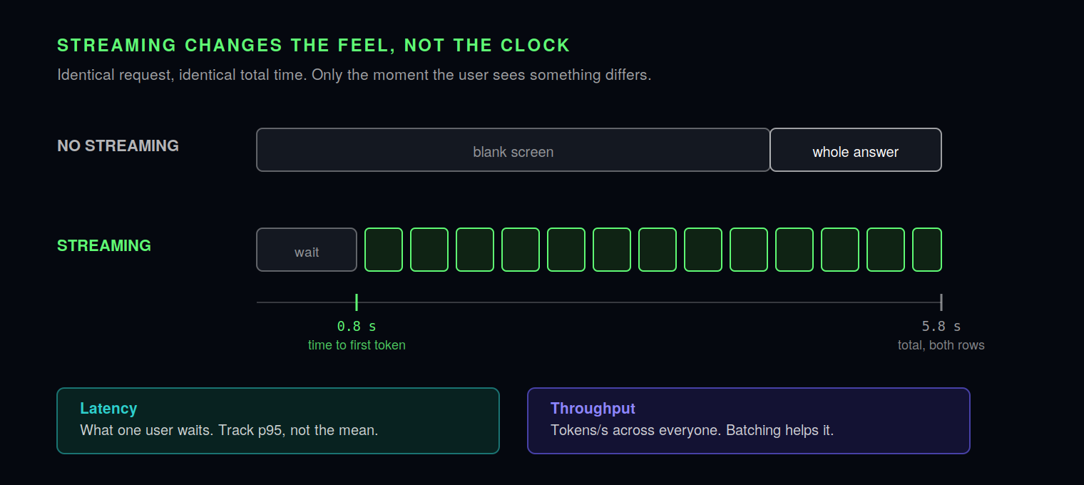
Both rows finish at the same moment. Streaming doesn't make the answer arrive sooner, it makes the waiting visible. That changes how slow the system feels while changing nothing about how slow it is. On modest hardware, streaming isn't a nicety, it is what keeps the thing usable.
Last thing, and it applies to all of the above: track p95 and p99, not averages. An average politely hides the requests that missed the cache, hit a cold model, or dragged in an unusually large set of fragments. Those are the requests your users remember.
Three places inference runs
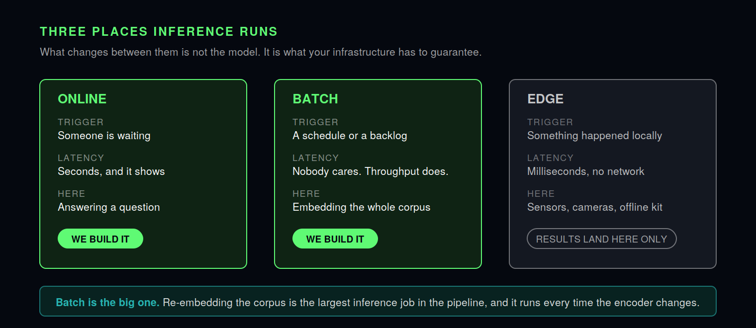
Our system runs the first two. Online when a question arrives, batch when the documentation gets indexed and again on every reindex.
Batch deserves more respect than it usually gets. Re-embedding a full corpus is the single largest inference workload in the pipeline, it runs every single time you change the encoder, and it is the operation that quietly decides whether your architecture can evolve later or is frozen on day one. Part 1 is built around making that replay cheap.
Edge doesn't appear in this series. Aiven's platform is where edge inference results land and get analysed, not where those models run.
Why not just fine-tune a model on the docs?
This is the first question everybody asks, so let's take it seriously. If we want a model that knows Aiven's documentation, why not train one on Aiven's documentation?
Three reasons, all of them practical rather than philosophical.
Fine-tuning teaches style much more reliably than it teaches facts. Train a model on documentation and it learns to produce text that reads like documentation. It does not reliably learn which configuration key sets which parameter. What you get is answers that sound authoritative and are wrong, which is strictly worse than answers that look uncertain.
Documentation changes every week. A fine-tuned model is out of date the moment someone edits a page, and the fix is another training run. With retrieval, an edited page is reindexed in seconds and the next answer already reflects it.
Fine-tuned models cannot cite anything. The knowledge is smeared across billions of weights with no path back to a source. Retrieval hands the model specific fragments, so answers come with links. For technical support that isn't a pleasant extra, it is the difference between an answer someone can check and an answer they have to trust.
So yes, the specialisation is real, but it lives in the system rather than in the model. The pipeline knows Aiven's documentation. The model knows nothing about Aiven and never will. Before every answer, the right pages get put in front of it.
The analogy isn't training a new hire. It is putting the right manual page open on the desk before every single question. Nothing is retained in between, and that is the design working as intended.
One exception, and it's a good one. Remember contrastive training, the pairs that taught the encoder what belongs together? Fine-tuning the encoder means running more of exactly that, on pairs from your own domain: real questions, and the passages that actually answered them. It measurably improves retrieval, and it is the defensible use of fine-tuning in a system like this.
The catch is that it needs data only a running system can produce. Part 2 comes back to it, because the pipeline generates exactly that dataset as a side effect of operating. Every answered question with a helpful rating is one more pair.
Hallucination, and how to make grounding measurable
Hallucination: a model stating something false with exactly the same confidence it states something true.
This isn't a bug waiting to be patched. A decoder produces probable text, and probable text is not the same thing as accurate text. That is the mechanism, not a defect in it.
Retrieval helps by changing the task. Instead of "tell me what you know about Kafka partitions", the model gets "answer this using the three fragments below". That is summarising supplied material, which models do far more reliably than recalling facts.
Helps, though. Not solves. The model can still blend a fragment with something it half-remembers, or answer confidently from fragments that turned out to be irrelevant.
Which is why the useful definition of grounding is a measurable one rather than a moral one.
Groundedness: every claim in an answer traces back to a retrieved fragment.
That is checkable. Automatically, by testing whether each claim is supported by the supplied text. Manually, by reading answers against their citations. And once it is checkable it becomes a number that moves when you change something, which is what separates a system you can improve from a system that merely demos well.
Refusal: the system saying the documentation doesn't cover this, instead of producing something.
Refusal rate is worth watching in both directions. Too high means retrieval is failing. Too low means the model is inventing.
Three words to be careful with
These three carry more weight in marketing than they do in engineering, and knowing what they actually denote will save you some disappointment.
"Agent" means a model that can call functions, gets the results back, and decides what to do next. That is a real and useful capability. It does not imply judgment, reliability, or autonomy in any strong sense. An agent querying your database is a model choosing between functions you defined and wrote.
"Reasoning" describes models trained to write out intermediate steps before answering. The mechanism is one you already know: every token is generated from everything before it, so steps the model writes down become context it can build on. It is thinking on paper, and it measurably improves accuracy on multi-step problems. That is a genuine result.
It is not deliberation, though, and those steps are not a faithful record of how the answer was produced. It is not free either. Every one of those steps is a completion token, the slow kind, so a model writing two thousand tokens of reasoning before a hundred-token answer takes minutes on modest hardware. It is also where quantisation hurts most, because a slightly-off step becomes the input to the next one. And it is not the same thing as searching several times. A model that looks something up, reads the result and decides to look again is the previous word on this list: an agent.
"AI-powered" tells you nothing at all about what a system does. Every component in this series is AI-powered by any reasonable definition, including the part whose entire job is chopping documents into fragments.
None of these are lies. They are compressions, and what compressions lose is precisely the part that tells you whether something will work. Next time you read that a system is agentic, the question worth asking is which functions it can call and what happens when one of them fails.
What comes next
You now have the vocabulary: encoders and decoders, tokens and embeddings, cosine similarity, retrieval-augmented generation, sampling, weights and quantisation, latency against throughput, online against batch, grounding and refusal.
Part 1 turns all of that into an architecture. Which services carry which part of the work, and the exact shape of the data moving between them. It also introduces the problem that makes this particular system interesting, which is what happens when the Aiven documentation and the upstream PostgreSQL® documentation give different, equally correct answers to the same question.
Part 2 builds it, measures it, and publishes the point where it stops working.
Get building: Start free on Aiven

Table of contents
- Four words people use interchangeably
- There isn't one model, there are two
- Tokens: the unit of everything
- Embeddings: teaching a search engine what you meant
- How the numbers get made
- Why similar meanings end up close
- What "similar" means, precisely
- What about other languages?
- One question, start to finish
- That has a name: RAG
- Three knobs that actually matter
- Quantisation: same model, less memory
- Why it feels slow, and what to measure
- Three places inference runs
- Why not just fine-tune a model on the docs?
- Hallucination, and how to make grounding measurable
- Three words to be careful with
- What comes next